


Intro to Strain Analysis: Techniques to Promote Measurement Accuracy
June 27, 2019Comments
The stamped-part-development process becomes more robust when strain analysis is used to ensure that stampings can tolerate the natural and inherent variation in mechanical properties of the ordered sheet metal. Techniques employed by strain analysis practitioners influence the results, and as a result, the conclusions drawn from the analysis.
| The metalforming industry lost a vocal advocate when Dr. Stuart Keeler passed away this past May. The Science of Forming was not just the name of the column he wrote for almost 20 years, (from 1999 through 2017), but a description of his many contributions to the field. Whether lecturing in a classroom setting or next to a stamping press in a tool shop, Stu highlighted the importance of using data in a field previously dominated by art. His leadership, passion and guidance will be missed. |
FLC0 is defined as the lowest point on the Forming Limit Curve and occurs at 0 minor strain. The Keeler equation for low-carbon steel can be used:
Equation 1
FLC0 = (23.3+14.2t) x (n/0.21)
where t represents sheet thickness (mm), and n denotes the n-value. In the example of a 0.8-mm-thick drawing steel with an n-value of 0.18, this equation determines FLC0 as 30 percent. Standard practice is to drop this value by 10 percent to account for the marginal zone, so we target a maximum value on the major strain axis of 20 percent.
This value must be put into perspective. In circle grid strain analysis, a flat metal sheet containing a grid pattern of 0.100-in.-dia. circles is formed and the circles flow into ellipses. Should a maximum major-strain value of 20 percent be allowed, then the locations that measure 0.120 in. on the long axis rest on the boundary of the safe/marginal zone. For this article, assume a minor strain of 0 percent, or plane strain, to make the math easier.
Compare that against an ellipse measuring 0.122 in., which falls into the marginal zone with a safety margin of 8 percent. An ellipse measuring 0.118 in. is graphed in the safe zone with a safety margin of 12 percent. This difference of 0.002 in. in either direction, assuming accurate measurements, makes the difference between tooling buyoff and tooling work.
The tools used to create the circles on the flat sheet and measure the ellipses on the formed part contribute to measurement accuracy. The circles typically are applied by electrochemical etching, which requires using a stencil of the correct grid pattern. The width of the line that forms the boundary of each circle measures about 0.008 in. A translucent Mylar strip calibrated to measure the expansion percentage of each circle also contains lines (the diverging railroad tracks) measuring about 0.008 in. thick.
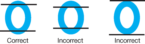 |
| Ellipse measurements using calibrated Mylar strips must be made from the center-width position. The width difference between the ellipse circumference and the diverging ‘railroad tracks’ in this image is exaggerated for clarity—in reality, they are of similar dimension. |
Accurate measurements require measurements from the center-width locations of the boundary line around the circumference of the ellipse. Inside-to-inside or outside-to-outside measurements are incorrect, as depicted in the figure, with an exaggerated difference in line thickness.
In the example targeting a 20-percent critical major-strain axis, measuring inside-to-inside (the middle example in the figure), the major strain axis reads as 0.112 in. (0.120 in. - 0.008 in.), which is +12 percent on the major-strain axis. Similarly, the minor-strain axis is measured as 0.092 in. (0.100 in. - 0.008 in.), which is -8 percent on the minor strain axis. On the other hand, a measurement of outside-to-outside dimensions (the righthand image in the figure), results in +28 percent on the major-strain axis and +8 percent on the minor axis.
In these examples, the boundary between the safe and marginal zone occurs at a data point of (+20 percent, 0 percent). Accurate measurements with an incorrect technique can lead to data points ranging from (+12 percent, -8 percent) to (+28 percent, +8 percent), and provides a false picture of the true situation.