
Page 44 - MetalForming March 2014
P. 44
When You Need it Fast
���� ����� � ����� �����
��� ������ ����� � ������ ����� ��� �����������TM �����������TM � ���������� ��������
In-Stock Items Ship in 24-48 Hours
Call us at
(513) 242-8900
or
1-800-543-1566 www.diehlsteel.com
Ready; Set; Lean
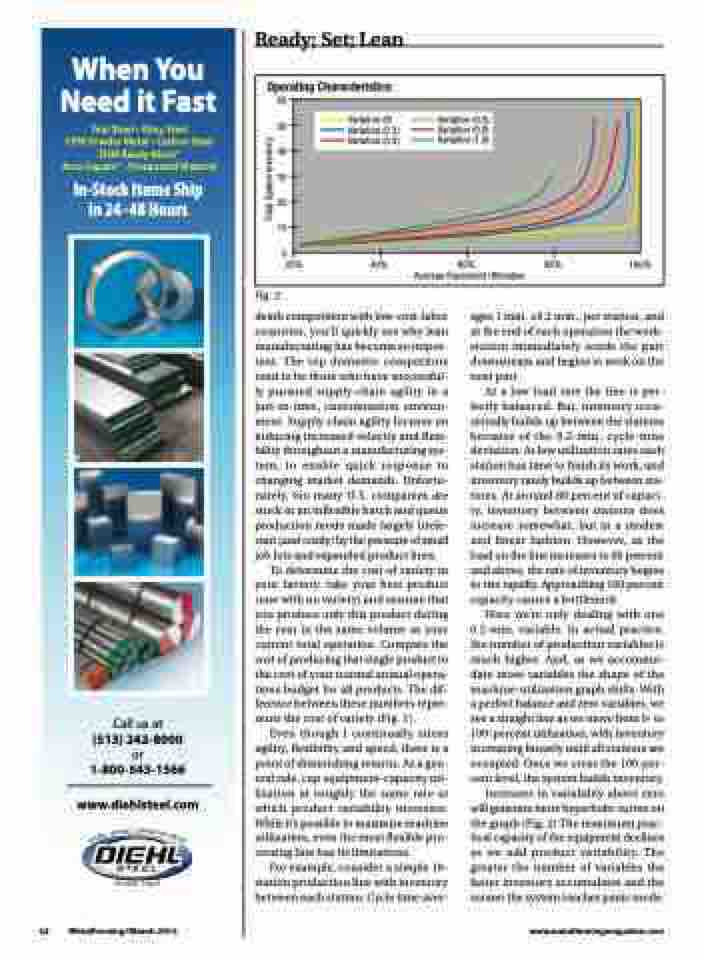
Operating Characteristics
60 50 40 30 20 10
0
20% 40%
60% 80% 100% Average Equipment Utilization
Variation (0) Variation (0.2) Variation (0.4)
Variation (0.6) Variation (0.8) Variation (1.0)
42 MetalForming/March 2014
www.metalformingmagazine.com
Fig. 2
death competition with low-cost-labor countries, you’ll quickly see why lean manufacturing has become so impor- tant. The top domestic competitors tend to be those who have successful- ly pursued supply-chain agility in a just-in-time, customization environ- ment. Supply-chain agility focuses on inducing increased velocity and flexi- bility throughout a manufacturing sys- tem, to enable quick response to changing market demands. Unfortu- nately, too many U.S. companies are stuck in an inflexible batch and queue production mode made largely irrele- vant (and costly) by the pressure of small job lots and expanded product lines.
To determine the cost of variety in your factory, take your best product (one with no variety) and assume that you produce only this product during the year in the same volume as your current total operation. Compare the cost of producing that single product to the cost of your normal annual opera- tions budget for all products. The dif- ference between these numbers repre- sents the cost of variety (Fig. 1).
Even though I continually stress agility, flexibility and speed, there is a point of diminishing returns. As a gen- eral rule, cap equipment-capacity uti- lization at roughly the same rate at which product variability increases. While it’s possible to maximize machine utilization, even the most flexible pro- cessing line has its limitations.
For example, consider a simple 10- station production line with inventory between each station. Cycle time aver-
ages 1 min. ±0.2 min., per station, and at the end of each operation the work- station immediately sends the part downstream and begins to work on the next part.
At a low load rate the line is per- fectly balanced. But, inventory occa- sionally builds up between the stations because of the 0.2-min. cycle-time deviation. At low utilization rates each station has time to finish its work, and inventory rarely builds up between sta- tions. At around 80 percent of capaci- ty, inventory between stations does increase somewhat, but in a modest and linear fashion. However, as the load on the line increases to 85 percent and above, the rate of inventory begins to rise rapidly. Approaching 100 percent capacity causes a bottleneck.
Here we’re only dealing with one 0.2-min. variable. In actual practice, the number of production variables is much higher. And, as we accommo- date more variables the shape of the machine-utilization graph shifts. With a perfect balance and zero variables, we see a straight line as we move from 0- to 100-percent utilization, with inventory increasing linearly until all stations are occupied. Once we cross the 100-per- cent level, the system builds inventory.
Increases in variability above zero will generate more hyperbolic curves on the graph (Fig. 2) The maximum prac- tical capacity of the equipment declines as we add product variability. The greater the number of variables the faster inventory accumulates and the sooner the system reaches panic mode.
Total System Inventory
